Idle math – MossGoblin

Fibonacci Magic Square Building Analysis

So…

After I’ve slept over it.

The Fibonacci works well, because the algorithm creates a base case with a ‘0’ MC.

The schema again:

C	-	B
-	0	A
-	D	-

C	-D	B
-A	0	A
-B	D	-C

I was just doodling last night and just kind of figured it out to make it work, but now that I look at it, it is obvious why it had to be this way.
Starting in order of the Fib numbers…
Ok, Ok, let’s do it properly.

F3	-F4	F2
-F1	0	F1
-F2	F4	-F3

Let us build it with a few simple steps.

So, three principles to the arrangement:

0. We place a zero in the middle.

1. We are considering the sides – the lines that do not go through the center. In order to bring each one of them to 0 using the Fib numbers, we simply take advantage of the fact that, by definition, we will get to 0 if we take any Fib number (2 and above) and remove the previous two. Meaning that we need two consecutive Fib numbers with one sign (positive or negative) and the next Fib number with the opposite sign.

1.1 We have 4 Fib numbers and we need them to cover 4 sides. The way to do it is to use the fact that 4 consecutive numbers form 2 overlapping subsets of 3 consecutive numbers each – F1 to F3 and F2 to F4.
Given that F2 and F3 are part of the two subsets, we place them in neighboring corners. Now F3 will form one of the subsets with F2 on their shared side and the other subset on the other side. Similar for F2.

F3	-	F2
-	-	-
-	-	-

1.2 From the subsets we know that F2 is the middle value in subset 1 and the lowest value in subset 2. Correspondingly, F3 will be the highest value in subset one and the middle value in subset 2. This means that the top side (in this rotation), that already contains F2 and F3, will be part of the two subsets.
This is where we note that at this stage we have four sides with a total of four copies of the two subsets. For now, we will forget about the sign of the numbers and focus on the values.
Once we have the F2 and F3 placed, the rest is almost automatic. We have one choice to make, which is completely arbitrary, because it gets cancelled later on by the symmetries of the MS.
We need to place either F1 or F4 between F2 and F3 that are already on the board. Let’s choose F4. This means that the newly formed side is the larger subset.
We copy each of the values across the center, resulting in another copy of the subset, just in reverse order looking in the same direction (from left to right in this case). Only two cells remain and we fill them in with the value we did not choose the last time. In this case – F1.
We get:

F3	F4	F2
F1	0	F1
F2	F4	F3

1.2 We pick a side and start multiplying by -1. The rule that governs the multiplication is what we mentioned earlier – in each of the subsets, the two smaller values have the same sign, which is also opposite to the sign of the largest value.
At the top we simply convert F4 to -F4. So F2 and F3 remain positive. This means that on the right F1 will have the same sign as the F2 and F3 will become -F3. On the left F3 is the highest value, so F1 and F2 there will be multiplied by -1. This also automatically takes care of the bottom row.

F3	-F4	F2
-F1	0	F1
-F2	F4	-F3

1.3 Sanity check – across the center each Fib number stands opposite its negative, so along with the zero at the center, so each diagonal results in a zero.

1.4 Versions – the only notable thing so far is that if we had chosen to place F1 at the top, instead of F4, we would have gotten a schema that is flipped along the F2 diagonal. It is not immediately obvious to me why F2 and not F3. Needs some looking into.

-F3	F1	F2
F4	0	-F4
-F2	-F1	F3

—

Consequence of this whole thing. We are not using the fact that the numbers are part of the Fibonacci sequence. We are merely using the property that numbers in the Fibonacci sequence have – each equals the sum of the previous two. Which means that we can also freely use the Lucas sequence or any other that shares the same building principle.

Next:
– What about Tribonacci? Can we extend the algorithm to cover 4×4 MS? There are some nice complications that are visible from the start – we will need longer Fib subsets, but we still have only four sides. Also, we have outer sides and inner sides. Delight!

Fibonacci Magic Square

So I was wondering about magic squares (pattern hunting, obv) and I tried going the way of the tipping table.

Meaning: There are infinite magic squares with the magic constant X. The most boring of all is the trivial one, where each square holds value X/3. So… How about a way of getting from the trivial square to a non-trivial one? Obviously there are many ways and obviously many of those ways have already been described somewhere, but it’s worth digging (I have mentioned the value of rediscovering the wheel, haven’t I?).

So I started poking at a ’15’ square and got something that at the time looked surprising (now – may be not so much).

Disclaimer One – I have only had time to look so far at the X/3 trivial case. Meaning – MS (tired of typing the whole thing out) with a constant (MC) divisible by 3.

Disclaimer One-and-a-Half: I would love to dig into rational MSs some day!

So… I took this MS from the internet:

8	1	6
3	5	7
4	9	2

That’s a ’15’ square, so it’s base case is all 5s.

And the question is: how do you get from all 5s to the one above?

It is clear that adding the same value to each of the cells does not break the MS, so first I thought of cutting down the slack – the lowest value is 1, so if we reduce each cell by 1… nothing special pops up.

Back there I mentioned the tipping table. Crude analogy, I admit, but bare with me.

If you have a trivial case and you push one of the values down, others will have to go up to compensate, right?

So… Let’s look at the difference table – a grid with the deviation of the actual MS from a trivial case I cooked up:

3	-4	1
-2	0	2
-1	4	-3

This only showed how… small and tame the MS is – the biggest absolute difference is barely below the trivial base value (5). It looked good. I needed a tame case to dismantle in peace.

So I played around in an electronic table (I was gonna say Excel, but it is not Excel), trying to see if I can find similar difference table or at least explain what makes this one work. Why 1 to 4? What other values would do the trick? Obviously, the rules of the MS will strictly dictate the arrangement of the values (and those rules should be examined further), but why those values?

Intermittent observation – this MS is of a family of MSs, where the center has 0 deviation. More on that later.

Not many minutes playing around later I stumbled upon a good family of MSs – the Fibonacci MSs. They are a subfamily of a larger one, of which the above example is a member of. The sequence 1, 2, 3, 4 is not a Fibonacci subsequence, but follows the same 0-center rule, so… until I dig into that particular example further, I consider them cousins to the Fibonaccis.

So! Yeah, the Fibonaccis (FMS)! Here is the end result, directly. Analysis – later.

Take the following schema (rotate as you please):

C	-	B
-	0	A
-	D	-

A, B, C and D here are four consecutive Fibonacci numbers. Once you place them, fill in the opposite cells with their negative counterparts.

At this point you have a ‘0’ MS. Also, you have negative values. To get rid of the negative values, add the largest (D) to each cell. This will set you up with a 0 at -D. If you dislike the zero, no worries – add any positive number to all the cells to produce any member of an infinite number of FMSs with the same difference table. Or ‘difference profile’. Yeah, that sounds better.

Example:

’34, 55, 89, 144′ turns into:

89	-	55
-	0	34
-	144	-

then into

89	-144	55
-34	0	34
-55	144	-89

Add 144 to raise the MS above the negatives:

233	0	199
110	144	178
89	288	55

You’ve got yourself a ‘432’ MS.
Add 1 to each cell and you’re up to 435.
And so on.

You’ve got an infinite family of magic squares, identified by the ’34, 55, 89, 144′ sequence. One caveat, though – since producing another family requires to add/remove 1 from each cell, the magic constants of all the families are divisible by 3, so… you’ll cover only the ‘/3’ infinity of magic sums.

All I need to do is write up the justification behind the arrangement of the seed Fibonacci numbers and… well, the link to the Fibonacci sequence is cool as well, so digging into that will also be fun.

Next:
– Why does Fibonacci work here?
– What’s behind the 1, 2, 3, 4 MS up there?
– Can we do rational MSs?

The sorting tree

After I stopped trying to improve on the performance of crystal sort (https://mossgoblin.com/sommath/2021/06/25/sorting-them-numbers/), I was left with the idea of the unused sorting algorithms.

See, the thing is, once the ball is rolling (the ball of finding the best solution of a problem, that is), it doesn’t stop to make sure it has covered all the path beneath it. In fact it doesn’t roll, it bounces. And wherever it touches the ground you have your next best solution. So a lot of ground never gets touched. You know how high the bar currently is and you know where you should start thinking onwards if you want to raise it even more. So, I think, there’s enough uncharted ground beneath that high performance bar for one to wander about.

Meaning – there are a lot of low hanging fruit to be picked, if you are so inclined. The point? Well, there’s exploration. That’s reason enough in and of itself. For me it is almost the same as finding yet another proof of the Pythagorean theorem. Not that anyone needs it, per se, but boy would I be proud if I found one!

I would not be as proud to find a relatively slow sorting algorithm, but it does please me enough.

Hence – Push Sort.

(to be properly documented and repo’d)

Again (as with crystal sort) I named it myself. Even though undoubtedly it has been by someone considered half a century (or more) ago, it is clearly not clever enough to be performing well, so it has sunk in obscurity.

It is a very brute force approach and I was surprised that it ranked in the middle of the test table – I gotta cite some data, but if I remember correctly it was somewhere around merge, I think. See the comparison algorithms I used in the readme of crystal sort’s repo (I reused the benchmarking base).

The idea is very simple – take the elements from the bucket one by one and move them into a sorted bucket, placing them in the correct place within all other already placed elements. Let’s say you choose to sort ascending. You take the next bucket element and compare with the first sorted element. If the new is smaller or equal, insert it there (place in at index 0 and shift the others). If it is larger, repeat comparison with the next. If there is no next, then you have the largest element so far, so place it at the end.

As I said – it works surprisingly well. No trailblazer, for sure, but still.

Anyways. I have more to say about the low hanging fruit, but I’ll leave that for some other time. May be with the next mediocre sorting algorithm.

P.S. I should start using pseudocode and code blocks here…

Sorting them numbers

So I got me a sorting algorithm.

I really wanted to create one, just for the exercise. Of course, I did not have any expectations for it to be especially efficient, as I presume all low hanging fruits have been picked.
Well, it turns out we’ve picked up all the extremely low hanging ones, then we learned to reach higher and now we’re trying to pick the high hanging ones, but I suspect there are still unpicked fruits on the lower end.

That’s where my algorithm stands. And a bit to the side.

What’s the situation – crystal sort (as I called it) is generally slow, except for when you have an array with a particular property and you know in advance that it has it (or you strongly suspect that it does).

Quick disclaimer – I spent about two hours googling sorting algorithms, trying to read the basics of all of them. I could not find mine amongst them. My suspicion is that many people have come up with the idea already, but have dropped it due to it’s shortcomings. I am happy enough with the idea even though it’s not optimal, so I’m trying to make the most of it. It deserves the light of day (some light of day), even though it’s not groundbreaking.

So… I was mulling over the general sorting problem (well, the linear sorting mostly, iterations + swaps) and I was thinking about the eponymous bubble sort, used for the “low bar” benchmarking (along with shuffle sort, I guess).
I was thinking about how we keep the bubble sort around as an example and that every time you look at it you have to ignore the obvious optimizations, just so that you have it remain a pure example. Specifically, I was thinking about how you always swap adjacent elements of the array, disregarding the question “does this swap put at least one of the elements in it’s correct position”. So I decided to code that as an exercise and to my delight I found that it’s performance is… not abysmal.

Generally what happens (or happened in that first version) is that you go through the array and compare your current element with the first and the last one. You swap it with the first one, if the current one is smaller. Otherwise, you swap it with the last one, if the current one is larger. Very, very simple, yet at the end of the pass you are guaranteed to have both the smallest and largest elements of the array at their exact correct and very final positions. Then you simply do the same for the remaining elements between them until you run out of remaining elements.

This proved to be so elegantly simple that I had to make an effort to “properly” code it – to be efficient, optimized and beautiful module. I did some comparisons (using ready-made code for other algorithms, lifted from the internet) and to my delight I found that it performed on par with selection sort (technically a tiny bit better, but within the efficiency margins that I suspect strict code optimizations govern; meaning – hard code overclocked code may cause the comparison to change a bit).

So… I was happy, but I realized the algorithm, as it was, had a major built-in inefficiency. Say you make one pass over the array and you get your smallest and largest elements at the first and last positions. Within the remaining elements you can have ones that have the same values, just scattered around. And in subsequent runs you’ll find them and place them where they belong, but the algorithm has no memory that it has already found those values, so… it seems like a missed opportunity. What if you could dispose of them quicker.

So I added another, secondary operation in between the primary iterations. After each primary pass, when you have found the min and max of the current subset, you go into the remainder and extract all values equal to those min and max and add stick them in their proper places. Then and only then you make another primary pass, finding new (and unique) min and max.

Result? Well, you have to consider the business case. Sorting algorithms are mostly used for small arrays with largely varying values. But if you, for some reason, want to sort an array that you know (or strongly suspect) has multiple duplicate values… well, then you better use insertion sort. But seriously, if you want, you can use my algorithm. It performs better and better the more duplicate values you have. In extreme cases (as I just suggested) it performs almost as well as the insertion sort.

For something botched together around almost non-existing expectations, I’m pretty happy.

Some disclaimers, again: The code that I used for comparison was lifted from https://stackabuse.com/sorting-algorithms-in-python
I presume the level of code optimization is the same between the different sorting methods (for a fair comparison between them), but also they are optimized for readability, as the blog post is supposed to be educational. So the different methods may turn out to have significantly different rooms for optimization, so if you choose performance over readability and refactor everything, the results may differ.
Also: The current code of my own algorithm is… well, I tried to keep it code neutral. Meaning I chose to keep an “iteration + swap” version, in order to exclude anything that is python specific. So it could be a bit faster with list comprehension.

Keeping that in mind, I can’t resist but try it that way – comprehend my lists to the max to see what would happen. I’ll add an update, once this is done and evaluated.

Last (apparently), but not least:

The algorithm is called crystal sort, because of the way the sorted values crystalize from the ends of the array towards the middle. It just reminds me of crystallization.

And yeah, here is the repo, actually 🙂

https://github.com/MossGoblin/crystal_sort

Squircle Resolved

At the end I had to give up on calculating my squircle by hand.

Two reasons

Unity gives an automatic way to approach the problem;
The tool Unity gives works with any (some kinds of any) type of shape, not only with geometrically correct squircles

I ended up using ray casting. I feel like I cheated, but.. that’s life. On one hand, I don’t have the nerve to develop the maths to deal with the problem myself, so… see reason 1. On the other hand, I have the consolation of working with shapes even better than a squircle.

Here’s how it goes:

You have a player somewhere on the map and a list of objects you want to track on your compass.

On the minimap you see the player himself. He always keeps his Noth-bound position, so when you rotate, you see the map rotating around you. Each trackable object (if not close to be seen on the minimap itself) is represented as an icon on the border of the minimap. The border is the ‘compass’.

You get the angle between the player forward position and the object in real world, then create an icon on the compass and place it on the compass, keeping the same angle between the up position of the canvas and the icon. The problem is the distance between the icon and the center of the minimap.

Here’s what you do – you have a secret object, outside of the playing area, that is basically a 3d version of the shape of your compass. That’s your ‘wall’. It’s hollow. In the middle there’s a radar object with a small script. You give that script the angle ‘in the real world’ between the player.forward and the object. The radar fires a ray at that angle and returns the distance to the wall at that angle.

You get that distance, scale it accordingly and give it to the compass.

If feels clunky to have a real world object that scans constantly to get the distance, but it undoubtedly works and it works with almost any shape, at that. The only limitation for the form of your compass and minimap is that the border can not swerve to an extend that one part of it blocks line of view from the center to another part.

Here’s the physical object with the (invisible) radar in the middle.

The radar is currently tracking 6 objects from the map, using angles, provided by the map itself. The visible rays are Debug.DrawRay().

Here are the map and the radar complex, set aside it:

You can clearly see that I haven’t even bothered to set the anchor points of the objects to the centers of their bases. I am tracking their basic 0,0 vertices here. Irrelevant.

Here are both the scene view and the play view:

All colored objects are on the compass. The compass itself is the blue band around the minimap.

This was just a feature-dev scene, so I didn’t bother matching colors of objects to icons. Black icons are blue objects. Yellow is yellow.

So… this has not yet been transferred to the main scene. In the full version you have multiple type of objects that you can see on the compass, some only from a certain distance. All of them should disappear from the compass if there are actually seen in the minimap (here you can see the yellow object bot on the map and the compass).

This step of transferring the compass success to a ‘main scene’ type of actual structure will be hell…

Uuhh!! Look what I found ShareX can do!

Screen recording! And – Tadaaaa! – Screen recording to GIF!

More on the line

(Continuation of Once a line, always a line.)

One thing I skimmed over is the way you translate the regular space into the discrete integer space that I used to place the integer objects in. That takes more effort that I can be bothered to apply here.

So, in the service of transparency and brevity, here’s a summary of the conclusions of the previous post:

Usually an integer is represented as a point on the number line (same as non-integers, but that’s irrelevant).
In a multidimensional space, that can be translated as a section of line, laying on one of the axis – one of the ends of the section is on the origin, the other is N units away, where N is the size of the integer.
The prime factorization of an integer can be represented with a multidimensional object.
1. The number of dimensions of the object equals the number of prime factors of the integer.
2. One of the vertices of the object lays on the origin and from there, on the axis of each dimension, there is an edge with length equal one of the prime factors.
Each such object is unique (because each prime factorization is unique)
The object representation of a prima number is always a line – a one dimensional object.

— — —

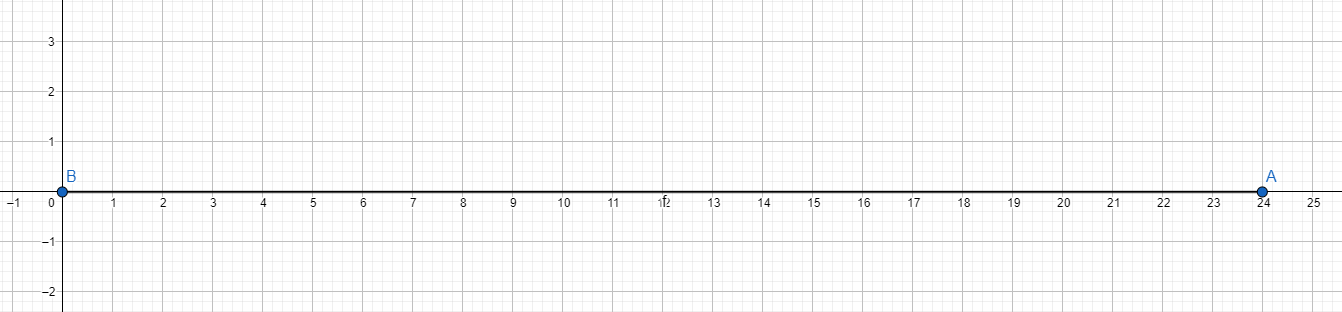
Here’s 24 as an integer on the number line:

…and here it is as a line:

…It could be a polygon:

… but that’s just regular factorization (one of).

The prime factorization of 24 is this:

This object can be only 24 and no other object can be 24 (rotations aside, because not relevant).

Once a line, always a line

I like primes. Particularly, among other things, I like the idea of them being building blocks for other numbers.

The problem comes from intuition mismatch – the operation that combines primes into numbers is multiplication, not addition. Admittedly, we are used to create by adding, not multiplying. Even more, we consider (and I can not think of a reason not to) that multiplication is a second order operation – an upgrade to addition.

So… I frequently turn the idea over in my head, trying to crack it and find a way to stuff it all in my intuition engine, so I don’t have to rationalize and accept it.

And a few days ago I had a kind of a break through. I can’t say that it’s something grand, but it’s a step in the right direction.

Prerequisite:

Since we are talking about prime numbers, we are working only in the realm of integers. So try to imagine the mathematical universe as a discrete place with a grid with granularity of 1. E.g. the smallest possible measurement is 1. or 1×1 in 2 dimensions, 1×1×1 in 3 dimensions and so on.

Then:

Consider the number 6.

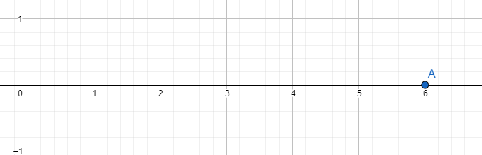
On the normal number scale it represents a point on the mark 6 on the positive integer axis:

This is the same as the distance between the point of number 0 and the point of number 6 on the integer axis. Like this:

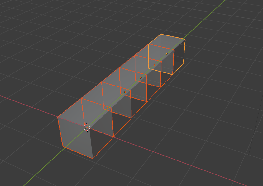
In the discrete integer space it looks like this:

The same, just showing the discreteness. This representation, going forward, is called the integer object of the integer 6.

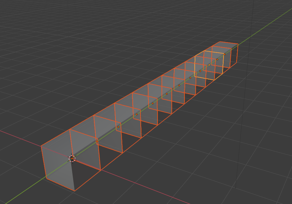
Let’s double it to a 12. Six would also do, but 12 gives a bit more options. So:

All fine and dandy, so far. 12 units laying on the X axis.

But we know we can represent 12 is a composite number – it has a prime factorization that includes more numbers than 12 and 1.

We can represent 12 as 6 times 2. Which, in a discrete geometrical sense, would mean extending the one dimensional integer 12 into 2 dimensions, creating an object of shape 6×2.

The reason I chose 12 is, of course, because its prime factorization is 2×2×3, e.g. it has 3 prime factors, so we can bring it up another dimension:

That’s the head of the idea that I had – that if you take the prime factors of an integer to be the size of an object in as many dimensions as there are prime factors, the compositeness of a number is very easy to grasp.

The important consequences of this representation (or what is this all about):

12 is 2×2×3 – there are two prime factors that are the same (2). This means that one of the cross sections of the object is a square. Not that it helps anything, but I thing it deserves mentioning.
- - Extending this would tell us that if we have n equal prime factors, there will be a cross section of the integer object that is an n-cube (if that is the proper term). Example: 24 is 2×2×2×3, so it can be constructed as a cube with side 2, extended in the fourth dimension to a length of 3.
So far so good. The next consequence is that an integer has a number of integer object representations – they equal the number of unique factorizations (mirrors exluded as not bringing any information to the table). Each representation, to be constructed, needs a number of dimensions, equal to the number of factors (in 2 dimension we can represent 12 sa 1×12, 2×6, 3×4).
Third – each object’s prime integer object representation has a minimum number of dimensions needed for it’s integer object to be constructed and that number equals the number of prime factors we constructed the integer from (for 12 we need 3 dimensions – for measures of 2, 2 and 3).
- Importnant – The number of prime factors of an integer determines the maximum number of dimensions we can meaningfully construct it in. For the integer 12, all dimensions above 3 do not bring any new information. Adding new dimensions after that will not change the relationship of the integer object to the space, as the shape itself can not have more dimensions. Meaning that in 4 dimensions, the 12 object will be a 3 dimensional object with a nominal 1 as it’s fourth measure.
And lastly – what is actually the heart of the idea – primes need only 1 dimension to exist. You can construct the integer object of a prime in a space with any number of dimensions, but only one of them will carry the information about the prime. All the rest will be nominal!

However many dimension you put 7 in, it will always be a line with length 7 – the most simple possible object with that size. In any number of dimensions (larger than 0) a prime number stays a line!

That is what I found fascinating!

And it comes back to the building blocks when you consider how the integer objects are created – one prime integer object aligned with the positive axis of each dimension of your space, all beginning at the origin.

Well… It turns out that even though the integers, as we usually think of them, are a single dimensional concepts, consisting of only a magnitude, but if you want to know how they are built – they are actually multidimensional objects. And for most of the integers those object representations have more dimensions that we are usually comfortable imagining.

P.S. Of course I could have done it with just lines and normal objects, instead of building it all out of blocks. But I think this way the discreteness is obvious at all times and in all representations and I find that to be the most important building block of the idea.

Biomes!

Aaand we have biomes!

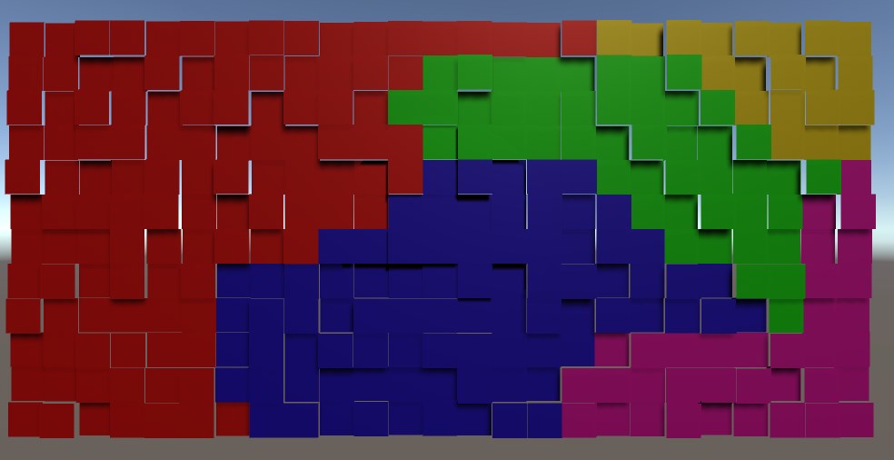
In this case they have only a visual role. The objects that the environment is constructed of have types and those are what is functionally important. I need the biomes, however, to mark different sections of the map differently. The players needs to be able to look at their minimap and determine that they are not in the same type of terrain.

The approach I took was to select points on the map that are generally far away from each other, then flood the area around each one. Of course, steady flood would mean straight lines between the biomes, so I had to think of a randomness.

I used random ‘height’. There is no height in the game, but the concept for randomization is height and I needed a visual distinction between the tiles while devving, so…

The idea is that in each iteration of the flood a tile is evaluated.

Each non-marked neighbour is marked for checking (pretty standard).

The check of the tile itself is a comparison of the height of the tile against a pre-set threshold. If the tile is low enough – it is marked with the color of the biome. If not – it is lowered by an amount and added back to the collection of ‘to be checked’ tiles.

And if you do it for each biome in turn, each with its own flood – it works!

We’ll see how it will break when I add it to the main scene 🙂

Enter Squircle

So… Remember how the players use glorified minimaps to actually play?

One of the main features of the minimap is the compass – icons, showing direction to points of interest.

Easy enough to do it on a circular compass. Found a way to do it also on a square one. The main concern is that the circle does not cover space well and I would be happier if I can allow the players top see more of their surroundings. Here comes the square minimap. However, square is not… friendly. I kind of don’t like the sharp corners. This can be, of course, mitigated, by designing the whole UI to accept such corners, but why mitigate a problem when you can resolve it?

Enter squircle – a square with rounded corners. It would look well and give more visibility than a circle with same radius as it’s side length. But how do you project icons on the compass?

The way the compass works is simple – you get the angle between the player forward direction and the direction to the object, translate that angle on the minimap and place the icon the right amount away from the center of the minimap. Yeah, that’s the problem. For the circle it’s basically a non-problem. For a square – I found a solution online (see below).

But a squircle? I think I found the correct road to a solution, but it’s still a rocky road for a person how has not practice any meaningful math for decades.

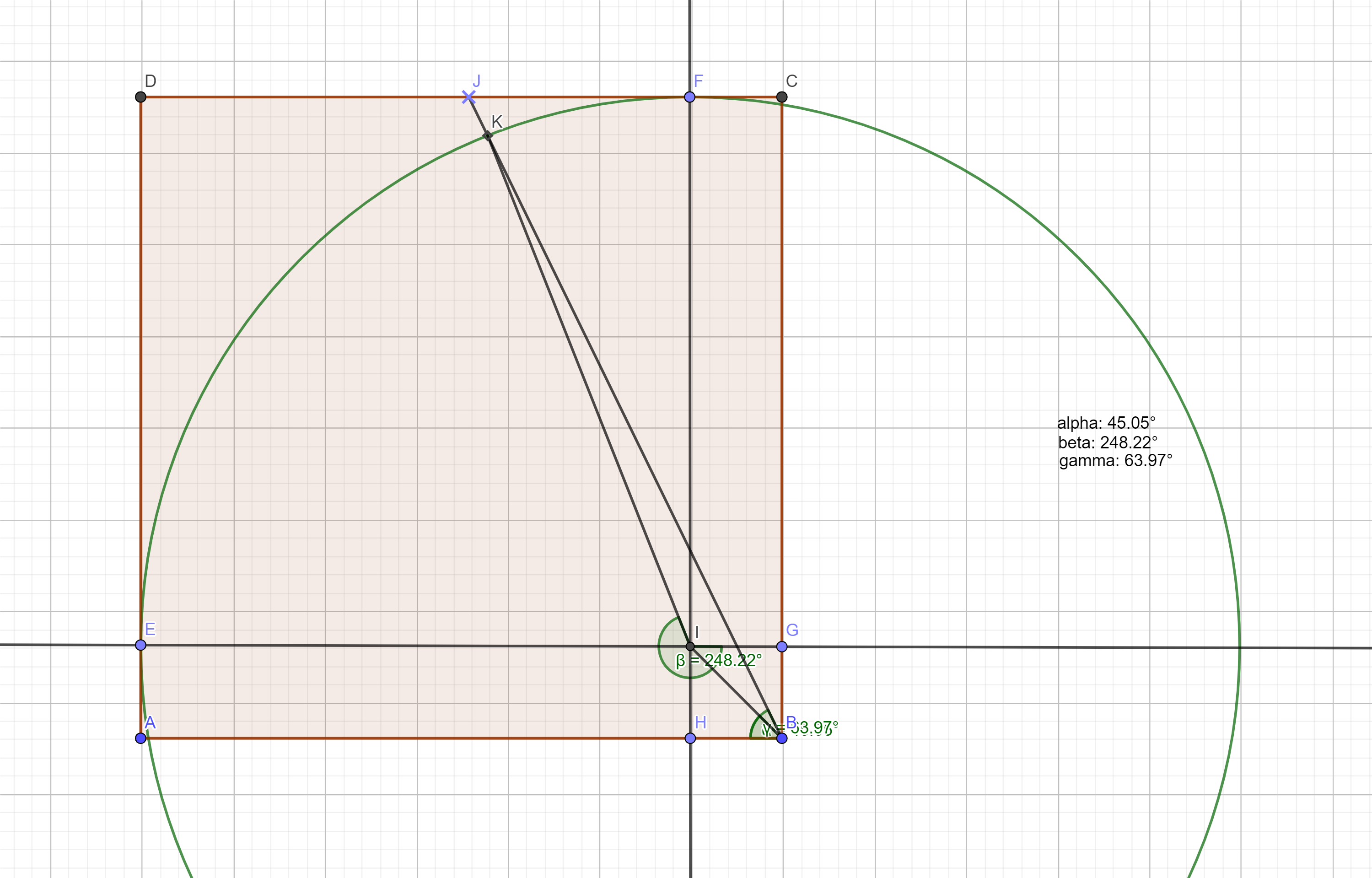
Here’s the construction:

The shape goes between two extremes. You have two governing variables – the radius of the corner circles and the length of the straight intervals between the corner circles. So the whole shape has two extremes:

it’s a circle if the intervals have length of 0
it’s a square if the radiuses are 0

What is given:

the radius of the circle
the length of the interval
the angle between (any) axis (IE) and the line passing through the center of the compass and the target icon (BJ)

What I need to find:

The angle between (any) axis (IE) and the line that connects the center of the circle and the crossection of the circle and the line from the center of the compass and the icon (IK)